
Understanding Black-Box ML Models with Explainable AI
XAI aims to enable the understanding of how Machine Learning and Artificial Intelligence work and what drives their decision-making.

With gaining popularity and their successful application in many domains, Machine Learning (ML) and Artificial Intelligence (AI) are also faced with increased skepticism and criticism. In particular, people question whether their decisions are well-grounded and can be relied on. As it is hard to gain a comprehensive understanding of their inner working after they have been trained, many ML systems — especially deep neural networks — are essentially considered black boxes. This makes it hard to understand and explain the behavior of a model. However, explanations are essential to trust that the predictions made by models are correct. This is particularly important when ML systems are deployed in decision support systems in sensitive areas where they impact job opportunities or even prison sentences. Explanations also help to correctly predict a model’s behavior, which is necessary to avoid silly mistakes and identify possible biases. Furthermore, they help to gain a well-grounded understanding of a model, which is essential for further improvement and to address its shortcomings.
Explainable AI (XAI) attempts to find explanations for models that are too complex to be understood by humans. The applications range from individual (local) explanations for specific outcomes of black-box models (e.g., Why was my loan denied? Why is the prediction of the image classifier wrong?) to global analysis that quantifies the impact of different features (e.g., What is the biggest risk factor for a particular type of cancer?).
When does an AI algorithm become a black-box model?
There is no definitive threshold for when a model becomes a black box. Generally, simple models with easy-to-understand structures and a limited number of parameters, such as Linear Regression or Decision Trees, usually can be interpreted without requiring additional explanation algorithms. In contrast, complex models, such as Deep Neural Networks with thousands or even millions of parameters (weights), are considered black boxes because the model’s behavior cannot be comprehended, even when one is able to see its structure and weights.
It is generally considered good practice to use simpler (and more interpretable) models in case there is no significant benefit gained from deploying a more complex alternative, an idea also known as Occam’s Razor. However, for many applications, e.g., in the area of computer vision and natural language processing, complex models provide higher prediction accuracy than simpler, more interpretable options. In these cases, the more accurate option is usually preferred. This leads to the use of hard-to-understand black-box models.
In contrast to the intrinsic explanations of simple models that are interpretable by design, black-box models are usually interpreted post hoc, i.e., after the model has been trained. In recent years, research has revealed many external methods that are model agnostic, i.e., they can be applied to many different (if not an arbitrary) ML models, ranging from complex boosted decision forests to deep neural networks.
An Overview of Explainable AI Concepts to Interpret ML Models
There are generally two ways to interpret a ML model: (1) to explain the entire model at once (Global Interpretation) or (2) to explain an individual prediction (Local Interpretation). Many explainability concepts only provide a global or a local explanation, but some methods can be used for both.
What is the rough overall consideration? — The Global Surrogate
The Global Surrogate is an example of a global interpretation. The overall idea is to train an interpretable ML model (surrogate) on the output of a black-box model. So, for instance, when using a Support Vector Machine (SVM) for a classification task, a Logistic Regression (one of the most well-known and studied classifiers), trained on the classification results of the SVM, could be used as a surrogate to provide a more interpretable model. This method is model-agnostic as any black-box model can be combined with any interpretable model. The interpretability, however, fully depends on the used surrogate. The important part is that the surrogate is being trained on the results of the black-box model. Therefore, conclusions can be drawn on the model, however, not on the data. The surrogate is usually not able to reproduce the results perfectly. This yields the question of when an approximation is good enough and whether some local decisions can be modeled sufficiently well.

Why this particular answer? — The Local Surrogate
In contrast to the global surrogate that attempts to substitute the black-box model as a whole, the idea of a local surrogate is to only approximate a part of the black-box model, which is a simpler problem and can be done more accurately. A well-known work utilizing this principle is LIME by Ribeiro et al. The general idea is to sample points around the prediction that should be explained and to probe the black-box model. The results are weighted based on their distance to the point to be explained since a local explanation is desired. Finally, a simple surrogate model is trained on these weighted samples, which is used as an explanation for the output given by the complex model for that very query point.
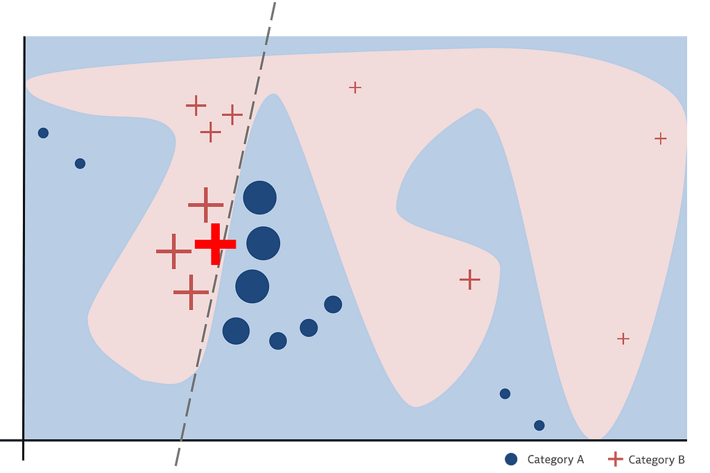
The advantage of this method is that it works for many different types of data (e.g., tabular data, text, images). Also, already simple surrogates lead to short and contrastive explanations as they only need to be valid for results close to the prediction that needs to be explained. However, defining the size of the neighborhood (i.e., assigning weights to the samples) is difficult. Another problem is that explanations cannot be considered stable. This means that two examples that only differ slightly may be explained quite differently, if the underlying model is very complex in that area, which makes it difficult to trust the explanations.
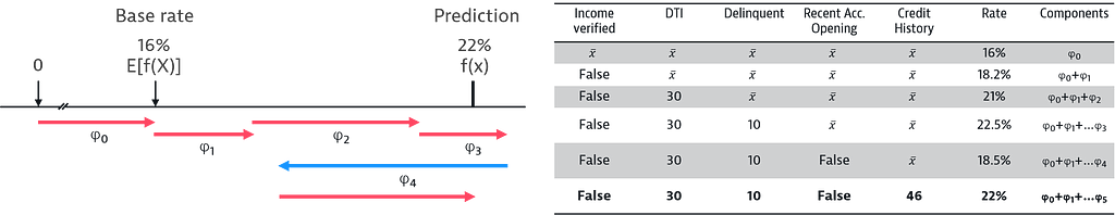
Which reasoning lead to this outcome? — SHAP
The need for stable explanations was an important motivation in the development of SHAP by Lundberg et al. Thus, it uses Shapley values — a concept from game theory — as a theoretical foundation. These were developed to fairly distribute payouts among participants in a coalition game. In the case of ML models, this idea is used to (fairly) assign the contributions of features to the output. This is achieved by first calculating a base rate, which refers to the model output when using the average of each feature as an input. One by one, this average input is replaced with an actual feature value to explain a specific prediction as shown in the figure below. The difference between the outputs when using the average across all values vs. the actual value for a specific sample is considered the contribution of this specific feature, which explains their impact on the overall result. However, since the contribution might differ depending on the order of how the features are filled, it is theoretically necessary to cover all possible orderings, which would lead to an unfeasible runtime complexity of O(n!). Addressing this performance issue is one major contribution of SHAP. The library provides ways to speed up and approximate these calculations to a degree where it is feasible to not just provide local interpretations of a specific prediction but also to repeat this process for multiple predictions to provide a global interpretation of a black-box model that allows investigating the impact of certain features on the model output.
This ability to provide local — explaining a specific answer — and global interpretations — the thoughts behind the model — based on a solid theoretical foundation is the major advantage of SHAP. The disadvantages are the high computational effort, which requires approximation, and the lack of a dedicated prediction model and feature reduction. Nevertheless, SHAP is a strong tool for investigating black-box models, specifically in domains that need reliable explanations and hence has already been adopted frequently.
Besides LIME and SHAP, which are two very well-known approaches, there are many alternative concepts. A more comprehensive overview can be found in the great book Interpretable Machine Learning by Christoph Molnar.
Whom to blame about that KPI change?
So, how does this connect to the challenges at Dynatrace? Dynatrace provides a powerful platform, which captures a large number of metrics. These are then automatically analyzed to identify anomalies and other issues. In the future, we envision that users can freely combine and aggregate these multidimensional metrics to define their own, custom Key Performance Indicators (KPIs). These KPIs themselves could then again be treated as time-based signals where automated analysis can be applied. If a problem is detected, a root cause analysis should be triggered to identify the source of the issue. However, due to the custom aggregation, the underlying problem, and thus the starting point for a further root cause analysis is unclear. Considering the custom aggregation as black-box model and the input signals as features allows for applying the previously discussed approaches of Explainable AI to this problem. They can help to identify the metric dimensions that have the most impact on the detected anomaly, which then are good entry points for a further root cause analysis.
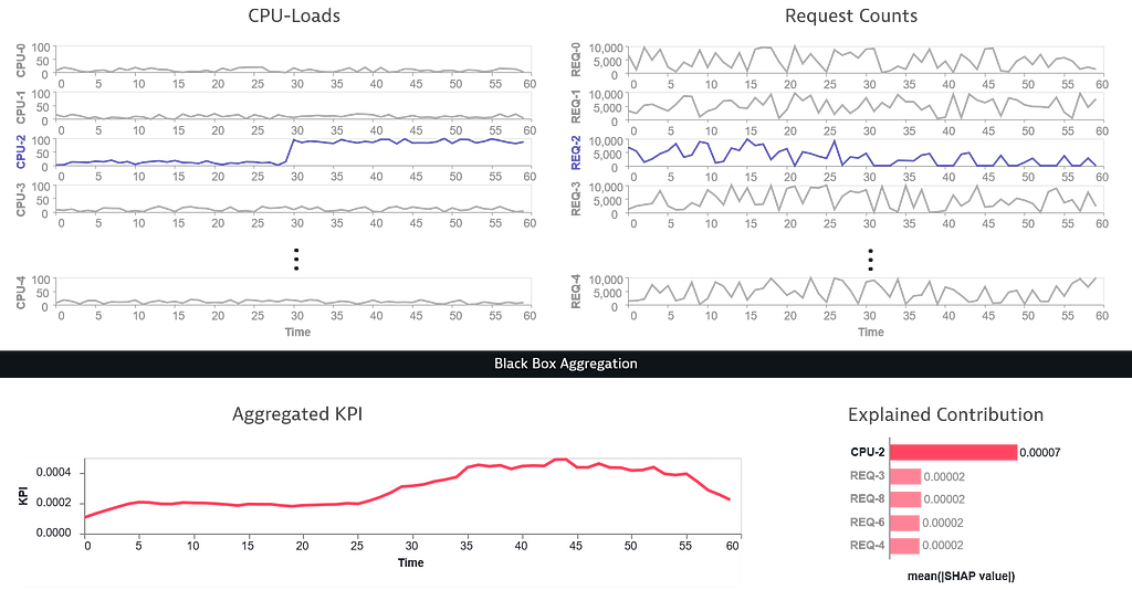
When only using simple operations and aggregations, applying perturbation-based approaches like SHAP is most likely not the most efficient way to gain these insights. However, the benefit of using methods from the Explainable AI toolbox in this scenario is that there are no restrictions regarding the creation and calculation of the KPIs, even if they involve ML methods. This way, it would provide a future-proof calculation method that does not need to be adopted when the capabilities for custom signal aggregation are extended.
The topics discussed in this article were also subject of a talk given at the University of Applied Sciences Upper Austria in March 2021.
Understanding Black-Box ML Models with Explainable AI was originally published in Dynatrace Engineering on Medium, where people are continuing the conversation by highlighting and responding to this story.