
Summarizing high-frequency latency measurements with strict error guarantees

High volumes of latency measurements are an issue that Dynatrace needs to deal with due to the nature of monitored services. Although there are some solutions out there, like HdrHistogram, they did not meet our needs so we developed our own data structure called DynaHist.
At Dynatrace we have to deal with high volumes of latency measurements, because monitored services are often called thousands of times per second or even more. Collecting and storing the value of every single response time measurement is not feasible at such high frequencies. However, without knowing them all, it is impossible to calculate percentiles accurately. This is a problem as latency SLOs are typically defined as percentile limits over some predefined period of time. The only option to reduce those high data volumes are data structures using lossy compression that are able to return at least approximate answers.
Since existing solutions did not satisfy our needs, we started developing our own data structure called DynaHist in 2015. After it was used for many years in production, it was recently published as a Java open source library.
Defining Tolerances
When dealing with approximate data structures, the question naturally arises what maximum error can be expected. There are two fundamentally different approaches for defining error tolerances in the context of percentiles. Both have pros and cons and are best explained with an example.
Let’s suppose that we are interested in the 90th percentile of the response time, and that the correct value would be 100ms if the original data were fully available.
The first approach would define the tolerance, for example, by requiring the approximative answer to lie between the 89th and 91st percentiles with a very high probability. This formulation already reveals the main problems of this approach. First, the limits apply only with high probability, which inherently makes it impossible to make absolutely certain statements. Second, the approximation error strongly depends on the distribution. If the 89th and 91st percentile values are far apart, the error might be very large. Examples of data structures based on this principle are the T-Digest, the KLL-Sketch, or the Relative Error Quantile Sketch. Since reliable statements are crucial for us, this kind of tolerance definition was out of question.
The second approach uses a simple property of ordinary histograms. The frequency counts of a histogram allow to locate the bin to which a value with given rank was mapped to. Therefore, the bin which contains a requested percentile can be straightforwardly identified. The bin boundaries obviously bracket the requested percentile value. As an example, if the 90th percentile (or equivalently the value with corresponding rank) was mapped to the bin covering the range from 98ms to 102ms, we know with certainty that the 90th percentile lies between both bin boundaries. Clearly, the maximum approximation error is given by the bin width.
By defining the bins appropriately, the relative error can be limited over a large value range. For example, to limit the relative error by 5%, we can just set the upper bound of every bin equal to the lower bound value increased by 5%. If we expect that all response times are all in the range from 1ms to 1000s, we would choose the bin boundaries according to the geometric sequence 1, 1.05, 1.05², 1.05³, …, 1.05²⁸⁴ (in milliseconds). Since the last boundary exceeds 1000s (1.05²⁸⁴ ≈ 1.04×10⁶), 284 bins will be sufficient to cover the whole value range while ensuring a maximum relative estimation error of 5% for any queried percentile value. If frequency counts are represented as 64-bit integers, the whole histogram would only take 2.2kB regardless of the original data size. The downside of this approach is that the expected value range must be known in advance to find proper bin boundaries. For latency measurements, however, this is not a big issue as the expected value range is usually known.
HdrHistogram
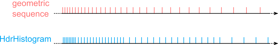
If bin boundaries are defined as geometric sequence, the mapping of a value to the corresponding bin will involve a logarithm evaluation. Since this is a relatively expensive operation on CPUs, Gil Tene (CTO and co-founder of Azul Systems) came up with a very clever idea, which he used for the very popular HdrHistogram data structure to achieve aggregation costs below 10ns per measurement. Compared to the geometric sequence, HdrHistogram sets the bin boundaries tighter so that the maximum possible relative error remains the same. In addition, the bin boundaries are arranged in such a way that the correct bin for a given value can be found with only a few cheap CPU operations. Tighter boundaries require more bins to cover a given value range, which also results in a space overhead of around 44% when comparing HdrHistogram with the geometric sequence for the same maximum relative error.
While we liked the basic principle of HdrHistogram, it did not satisfy all our needs. A major concern was that there is no free choice of the relative error. You can only select the number of significant digits corresponding to relative errors that are powers of 10, like 10%, 1%, or 0.1%. Furthermore, the error cannot be explicitly defined for values close to zero. A relative error limit is not suitable for them as it would lead to very small bins. We also missed the support for negative values and that minimum and maximum values are not tracked exactly. Because of all those reasons, and also because we came up with an idea to set bin boundaries with just 8% space overhead while achieving comparable update times, we decided to develop our own library called DynaHist.
How DynaHist works
A key feature of DynaHist is the easy configuration of a bin layout, because the bin boundaries are derived from four very intuitive parameters:
- Two parameters define an absolute and a relative error which you are willing to tolerate.
- The other two parameters specify the lower and upper bounds of a value range.
DynaHist ensures that every recorded value within the given range can be approximated with a maximum error that satisfies either the absolute or the relative error limit.
Let’s look at an example
The following example demonstrates how these four parameter values can be found in practice.
Let’s assume we want to collect the response time data of some service. We know that the resolution of the measurement is 1ms. Therefore, we can safely choose 0.5ms as absolute error limit, since it does not make much sense to be much more accurate than the resolution. Furthermore, we are fine with estimating percentiles with a relative accuracy of 5%, which gives the relative error limit. For response times, it is also easy to define the value range as they are inherently nonnegative and usually also bound by some timeout.
For example, setting the range to [0, 3600s] ensures that any response time of less than one hour will be recorded with either a maximum absolute error of 0.5ms or a maximum relative error of 5%.
The bin configuration finally defines the maximum array size that is internally used for storing frequency counts. For typical bin layouts the number of bins is in the order of hundreds or thousands. DynaHist has two histogram implementations allowing to choose between static and dynamic array allocation. The static histogram implementation allocates the maximum array size upfront and ensures allocation-free aggregations yielding highest performance. The dynamic histogram extends the array as needed to cover all nonempty bins. In addition, the number of bits used for representing frequency counts is adjusted dynamically. Possible values are 1, 2, 4, 8, 16, 32, and 64 bits. As the frequency counts of all bins can often be represented with less than 32 bits, this approach may result in significant space savings.
Benchmarking DynaHist and HdrHistogram
We ran some benchmarks comparing the static and dynamic flavors of DynaHist with the HdrHistogram version accepting floating-point values (DoubleHistogram). For both we used a comparable setup with a maximum relative error of 1%.
The results given in the figures below show that DynaHist outperformed HdrHistogram significantly. For the considered scenario (see here for the details), both DynaHist variants were able to record values faster using less memory.
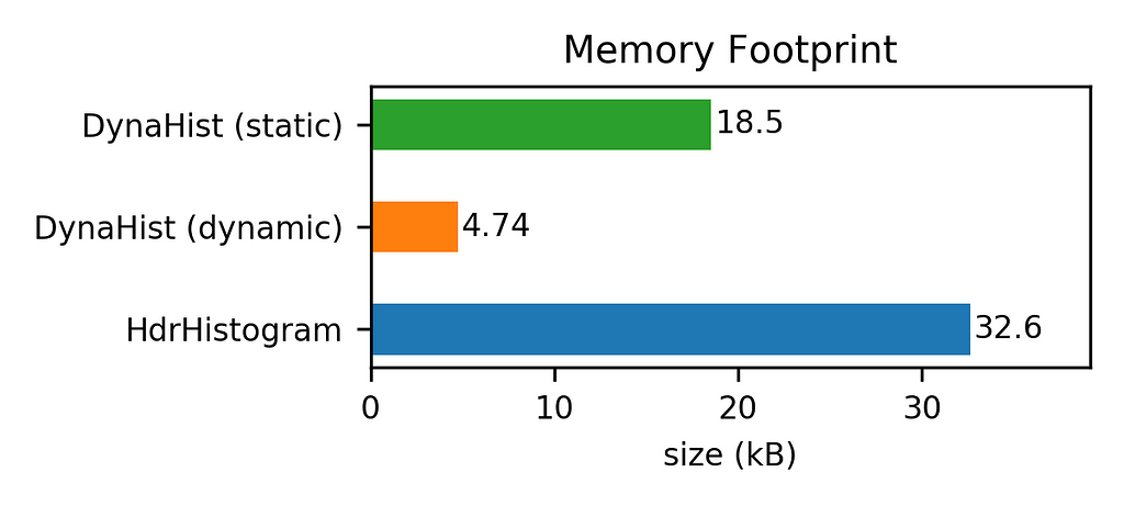
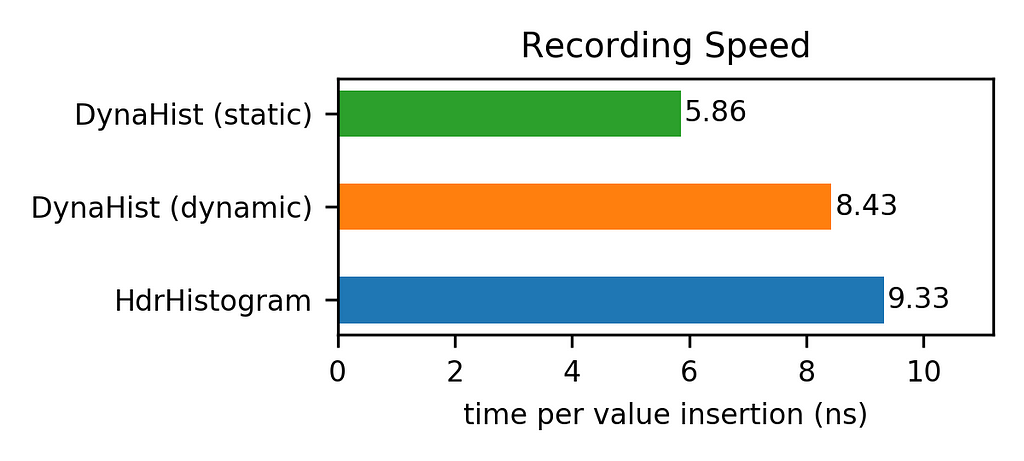
While the speedup was moderate, the savings in memory can be huge. In particular, the memory footprint of the dynamic version of DynaHist was only 15% of that of HdrHistogram. The reason for this is the more compact in-memory representation of frequency counts as well as the better choice of bin boundaries.
Summary
DynaHist is well suited to record and summarize latency measurements at high frequencies with low CPU and memory overhead while providing strict error guarantees for percentiles. If we have caught your interest, the Apache 2.0 licensed Java library can be found on GitHub.
Summarizing high-frequency latency measurements with strict error guarantees was originally published in Dynatrace Engineering on Medium, where people are continuing the conversation by highlighting and responding to this story.