A Deep Learning Approach for Network Anomaly Detection

Using modern deep architectures and domain adaptation techniques to differentiate between different anomalous activities.

Authored by José Arjona-Medina, Markus Gierlinger, Mario Kahlhofer, Hamid Eghbal-zadeh, and Bernhard Lehner.

Anomaly Detection (AD) can be defined as the identification of rare events, with respect to what is considered a normal event, often computed from a baseline. Network Anomaly Detection (NAD) refers to the identification and classification of suspicious network behavior or attacks.

Flow-based intrusion detection can be addressed with statistical methods, machine learning, or other techniques (Umer, 2016; Buczak, 2016; Bhuyan, 2014). However, classical machine learning approaches fall short when it comes to the ability to adapt to the complexity of the traffic, and the need to detect more complex patterns (Shahbaz, 2020). Motivated by the success of Deep Learning (DL) in other fields, DL-based approaches have seen an increased adoption for security-related tasks such as network traffic classification (Shahbaz, 2019). However, most of these DL-based approaches still struggle when labels are not balanced or in presence of distribution shift between training and test datasets.

In the following, we describe our approach which combines modern deep neural architectures, state-of-the-art domain adaptation, and regularization techniques to overcome the challenges of NAD. Our approach was evaluated in the NAD 2021 challenge, which was held as part of the ICASSP 2021 conference. Our best submission achieved a score of 0.3866 and placed 8th on the leaderboard.

The NAD 2021 Challenge

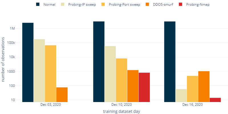
The NAD 2021 Challenge dataset consists of real network traffic recorded by © ZYXEL firewalls. Each one of the almost 10 million observations hold 21 features on a single network flow. This includes a timestamp, source and destination addresses and ports, connection durations, inbound and outbound traffic counts. Anomalous observations, which make up about 1 % of the data, identify probing attacks (port sweeps, ip sweeps, nmap scans) and DDoS smurf attacks.

The dataset consists of 3 days of network flows with labels (training dataset) and 4 days without labels (test dataset). Each day has a noticeably different feature and label distribution.

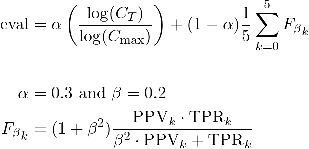
Final models are evaluated on the test set according to the following formula and confusion matrix, where C_T is the total cost (off-diagonal weighted sum of the confusion matrix), C_max is the maximal cost (maximal cost value of 2 multiplied with the confusion matrix), and F_beta_k is the F_beta score for class k.

Feature Engineering

You can take a glimpse at a small sample of the raw data here.

We extracted a total of 113 features, consisting of the following:

• All of the raw features, except time, src, dst, spt, dpt, duration, in_bytes, out_bytes, proto, app
• A one-hot encoding of all proto values (icmp, igmp, tcp, udp) and some app values (http, https, ftp, ssh, icmp, snmp, domain, ssdp, others)
• A one-hot encoded column if one of the following values is zero: duration, in_bytes, out_bytes, cnt_serv_*
• A log-transform of duration, in_bytes, out_bytes, cnt_src, cnt_dst, cnt_serv_src, cnt_serv_dst
• [ip_area] A one-hot encoding if the src and dst address belongs to the global, link-local, or unspecified region
• [ip_flow_type] A one-hot encoding for internet, intranet, ingress (from public to private), and egress (from private to public) traffic
• [ip_binary_match] The number of bits that are equal in the src and dst addresses from left to right, which quantifies how similar two addresses are
• [ip_one_bits] The number of set bits in src and dst, as a heuristic to identify broadcast addresses
• [port_area] A one-hot encoding if the spt and dpt ports belong to well-known, registered, or ephemeral port regions
• [port_match] A bit that is set if the spt and dpt port match
• [cnt_ratios][in_out_ratios][cnt_distances] Various ratios and distances among some features
• [segments] Our segment features which compute some features for some grouped ip flows

You can find our feature implementation right here.

Segment-based Features

The features on network flows already provide aggregated metrics of the packets that make up a connection. However, many of the attacks in our dataset originate from a single attack machine and may target an entire subnet. For example, it would be a good indicator for IP sweeps if we identify a single source address that tries to open connections to a huge number of target addresses.

Therefore, we first group our data by their source address and target subnet (i.e., the first three octets of the destination address, as a heuristic for that). Per group, we join flows that are temporally close and call them segments. In other words, we join individual flows to the same segment if any of the flows is less than 1 minute apart from another. As seen in the example below, given network flows at times [1, 2, 3, 7, 8, 9, 10, 15] in one group, we would create the segments [[1, 2, 3], [7, 8, 9, 10], [15]].

For each segment, we compute its length, and its number of unique destination addresses, source and destination ports, and app values. We assign these metrics to each individual data point as a new feature.

Group-based Splitting

Due to the nature of our data, traditional splitting methods might leak label information through some specific features. This is because many data points belong to the same session and therefore some features are shared among different points.

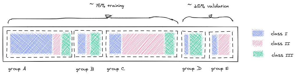
To avoid this leakage, we make sure that data points from the same session remain together, either in training or validation datasets. Therefore, we again group our data by their source address and target subnet and try to sample entire groups for each fold, while preserving the overall class distribution in each fold and achieving the desired size of the validation set (e.g., 25 % of the original data size).

The example in Fig. 4 shows one possible configuration to assign five groups into two folds, where each group has a different class distribution but the overall class distribution in the 75 % training set and 25% validation set is almost equal.

You can use our splitting-implementation for your project as well, which just brute-forces various group assignments until the desired ratio and class distribution is achieved.

Domain Adaptation

Model training and selection in supervised learning are often done by splitting the available data into training, validation and test sets. The underlying assumption is that all three datasets come from the same distribution. However, in real-world applications (such as the NAD 2021 challenge), this assumption is likely violated. This problem is known in the literature as domain shift or distributional shift. Domain Adaptation (DA) is the field that addresses this issue.

DA considers that training (source) and test (target) data might come from different (but related) distributions. DA generalizes to the problem of training from one or more source distributions to perform well on a different, but related target distribution.

When using neural networks, one approach is to align source and target domain distributions in a latent space, aiming at learning a domain-invariant latent representation. Central Moment Discrepancy (CMD) was recently introduced as a metric based on the sum of differences of high order central moments between the source and target latent activation space. We use CMD as a regularization term in the learning objective when training our network.

Multi-task Learning

Learning a model to optimize a particular metric is often done via minimizing an error function associated to that metric. By focusing just on that error function, a critical source of inductive bias for real-world problems might be ignored (Caruana, 1993). In classification tasks, the cross-entropy is often used as error function where for each sample only one of the classes is the target (single task). In multi-task classification however, every sample may have more than one target (multi-task).

In our multi-task models, we use various classification heads to individually optimize the loss w.r.t. a certain class (e.g, nmap scans), while an additional multi-class classification head, which is one of the jointly-optimized tasks, is used for the final prediction.

Self-normalizing Architectures

Normalizing the network’s input is a standard procedure in training neural networks. However, the normalization properties are often degraded after each layer’s output. Batch normalization (BN) has become a standard method to alleviate this problem, normalizing neuron’s activation for each training mini-batch. As a result, learning is more stable and faster since higher learning rates can be considered. Additionally, layer normalization or weight normalization are approaches to address this issue.

Recently, Self-Normalizing Neural Networks (SNNs) have been proposed to normalize neuron activations by incorporating Scaled Exponential Linear Unit (SELU) nonlinearity. Besides having a similar normalization effect as BN, SNNs are also robust to stochastic perturbations such as Stochastic Gradient Descent (SGD) or stochastic regularization methods such as Dropout or Shake-Shake, among others.

Architecture Regularization

To improve the robustness of our model, we opted for regularization methods that improve generalization onto shifted distributions and provide more robustness by built-in regularization mechanisms.

More specifically, we apply dropout on the neuron-level, and Shake-Shake regularizations on the gradients of the pathways in the residual connections in our architecture.

Hyperparameters and Architectures Selection

In our submissions, we use a deep SNN with Shake-Shake regularization in the backward pass and dropout of 0.2. We use the Adam optimizer with a learning rate of 3e-3. We split the available data into training and validation set, keeping almost the same distribution of label class. Model selection was carried out by early stopping, based on the performance of the evaluation criteria in the validation set. To tackle the label imbalance, we used a weighted sampler when feeding data to our batches.

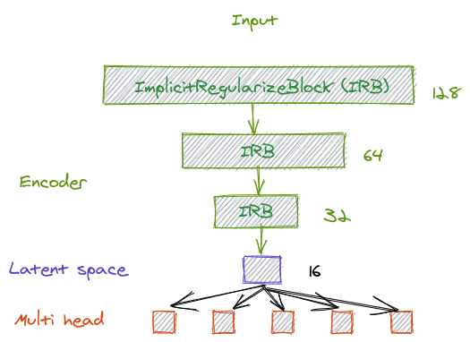
The chosen architecture consists of a 4-layer encoder, which outputs a latent representation. This latent space serves as input for the different prediction tasks (see Fig. 5).

Results and Discussions

We trained our architecture for 50K updates and 3 different seeds to average out any randomness introduced at the initialization. Plots below show the smoothed average over the 3 different runs.

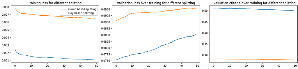
In our first experiment, we confirmed that splitting the data based on the day the data was collected results in a poor performance (both losses and evaluation criteria) compared to our group-based splitting approach (see Fig. 6).

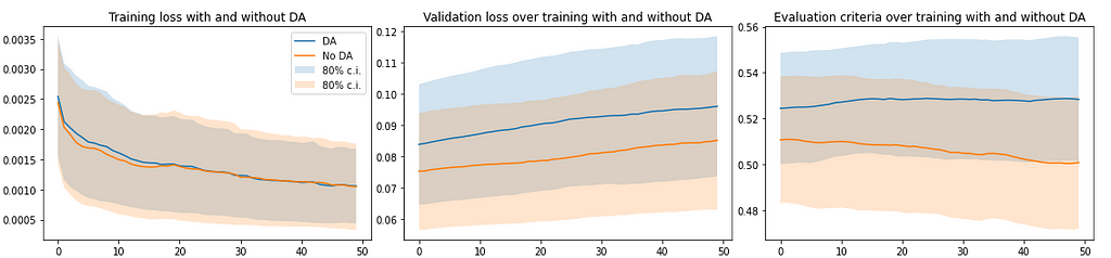
In a second experiment, we trained our architecture with and without CMD regularization loss using the group-based splitting. Fig. 7 shows how using DA improves the performance measured by the evaluation criteria. Shadows represent the confidence interval of 80%. Fig. 7 also shows the discrepancy between the validation loss and the evaluation criteria. An increase in the validation loss would suggest that the model is overfitting and hence, the evaluation criteria should decrease. However, when using DA, this effect is not shown. This indicates that the loss function could be further improved to optimize the performance criteria.

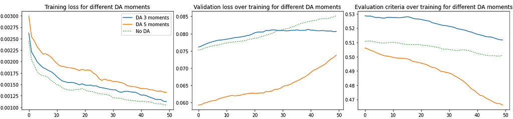
We further investigate the role of DA by trying different weights and different number of moments. Fig. 8 shows results for three different weights configurations and Fig. 9 for different number of moments.

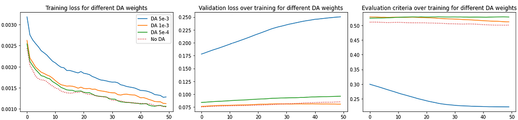
We can observe that applying DA improves overall performance, evidenced by overfitting prevention and a better average performance (evaluation criteria) across different seeds. However, the variance across the 3 seeds is still high, which could be resolved by increasing the number of seeds or increasing the number of validation samples.

Visualizing Network Flows

Unlike other data types like images, text or audio, it is not obvious how to visualize and inspect network flow data. While we cannot possibly visualize all of it, we tried to focus our attention on three main aspects: groups of network flows, their temporal occurrence, and the class labels.

Like before, we first group each individual data point by some grouping criteria, and its timestamp. We draw each group as a dot on a two-dimensional canvas, where rows (i.e., the vertical axis) indicate time, and each column holds one group. We color each dot by the majority label within its group. The order of the horizontal axis is arbitrary and doesn’t convey any meaning.

Let’s see an example. Fig. 10 shows the training data from Dec 3, 2020, grouped by source and destination port pairs, with port sweeps tinted yellow and the rest tinted grey. A port sweep shows the behavior that one source port is connecting to multiple destination ports. With this grouping, we can clearly spot the time blocks at which the port sweeps occurred.

Fig. 11 is a visualization of the detected port sweeps in the test data from Jan 23, 2021, as labeled by our ensemble model. As we see, it seems to correctly identify a quite similar pattern.

For reference, the following image shows the chaotic pattern a faulty model would produce. Fig. 12 shows the test data from Jan 25, 2021, tinting each one of the five classes in a different color.

This type of visualization can also be used to identify other attack patterns, if you change the grouping, e.g. to the source and destination subnet pairs. We used this visualization to sanity check all our model results. If you want to use a similar visualization for your data, you may experiment with our code that creates this with the help of HoloViews and Datashader.

Conclusion

In this work we showed that using modern deep architectures and domain adaptation techniques can successfully differentiate between different anomalous activities.

Experiments showed that splitting data points from the same session into training and validation datasets results in poor performance on the evaluation criteria due to overfitting. Considering session information when splitting the data showed better performance. Moreover, we observed that Domain Adaptation helps in preventing overfitting, yielding a higher performance. We also observed that the loss function could be refined to better express the evaluation criteria.

We experienced a notable disagreement between the validation score and the final test score, calculated by evaluating models on a set of unseen samples. We believe that our validation dataset has a large distribution mismatch with respect to the test dataset. However, since labels for the test data are not available at the time of writing this blog post, we couldn’t test our hypothesis. Future research will focus on constructing a validation set from the training data that faithfully represents the distribution in the unseen test.

This work is the result of a collaboration among Dynatrace Research, Silicon Austria Labs, Linz Institute of Technology AI Lab, and the Institute of Computational Perception, at the Johannes Kepler University of Linz.

A Deep Learning Approach for Network Anomaly Detection was originally published in Dynatrace Engineering on Medium, where people are continuing the conversation by highlighting and responding to this story.